Variance: The average squared deviation from the mean.
Standard Deviation: Square root of the variance.
# Rangerange(data)
[1] 5 10
diff(range(data)) # Range as a single number
[1] 5
# Variancevar(data)
[1] 2.527778
# Standard Deviationsd(data)
[1] 1.589899
📈 Data Visualization
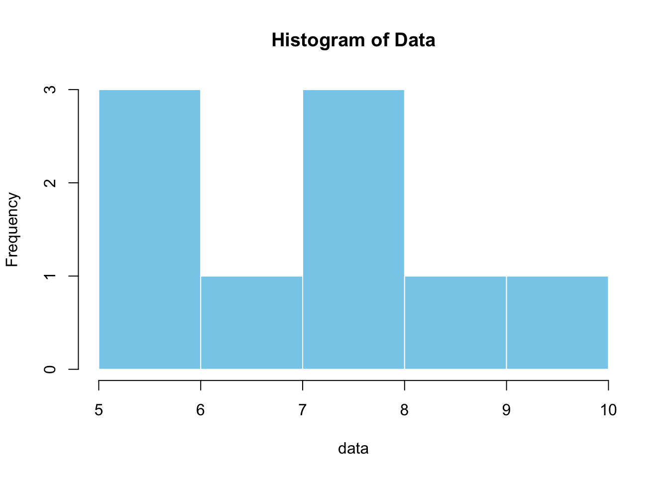
Visual representations are essential for understanding the distribution of data.
# Histogramhist(data, main ="Histogram of Data", col ="skyblue", border ="white")
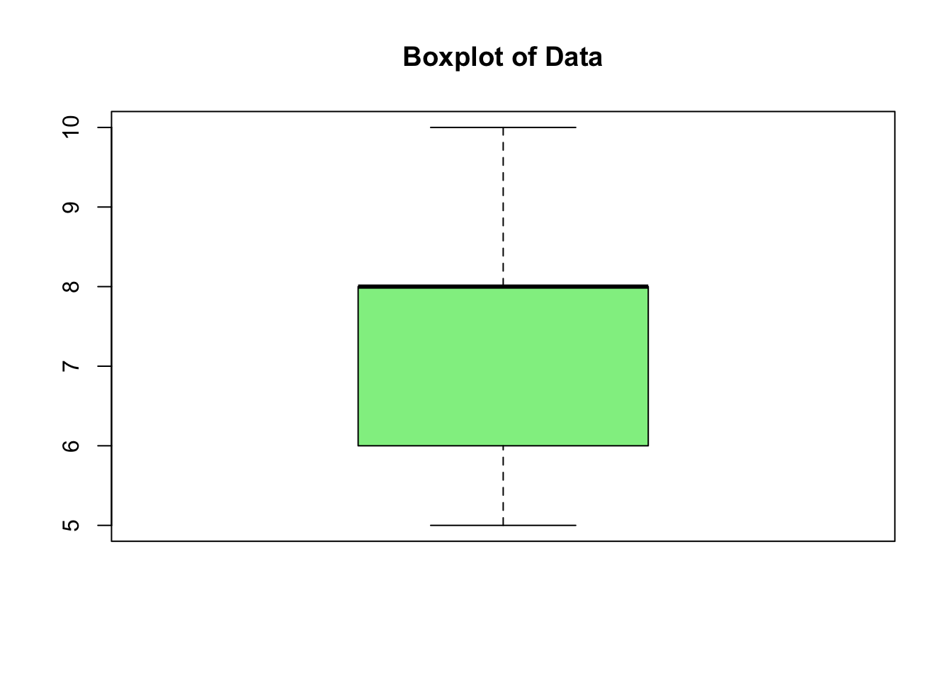
# Boxplotboxplot(data, main ="Boxplot of Data", col ="lightgreen")
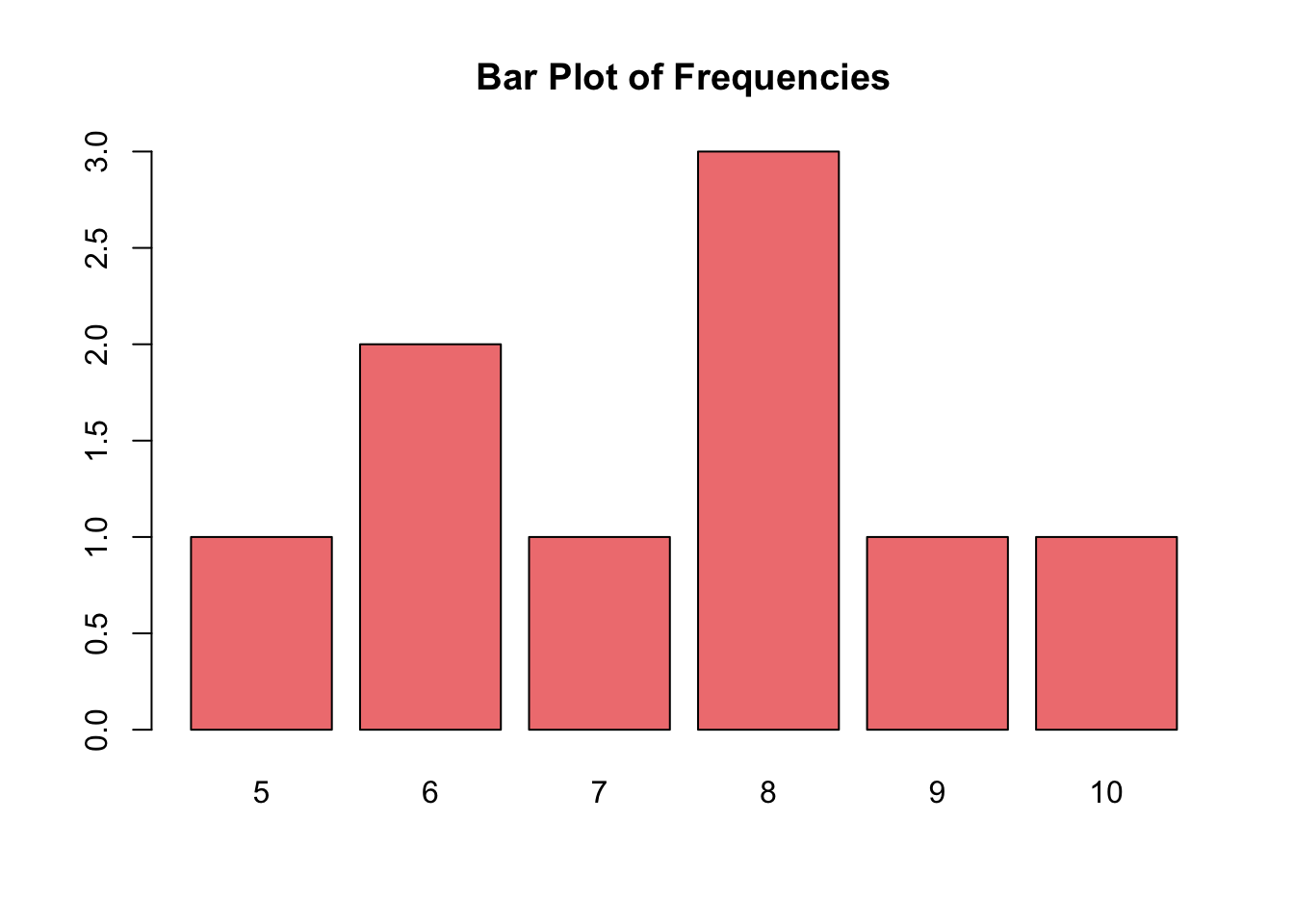
# Bar plot for frequencybarplot(table(data), main ="Bar Plot of Frequencies", col ="lightcoral")
✅ Summary
Descriptive statistics give you a first understanding of your data. You can use these techniques and R code snippets to quickly explore any dataset before moving on to more complex analysis.